No Reference Metrics
Demonstrates the use of the no-reference metrics: NPS, MTF, and NEQ.
from xdesign import *
import tomopy
import numpy as np
import matplotlib.pylab as plt
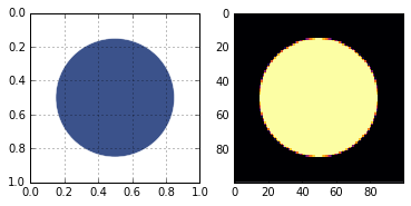
Generate a UnitCircle test phantom. For the MTF, the radius must be less than 0.5, otherwise the circle touches the edges of the field of view.
p = UnitCircle(mass_atten=4, radius=0.35)
sidebyside(p, 100)
plt.show()
Generate two sinograms and reconstruct. Noise power spectrum and Noise
Equivalent Quanta are meaningless withouth noise so add some poisson
noise to the reconstruction process with the noise argument.
Collecting two sinograms allows us to isolate the noise by subtracting
out the circle.
np.random.seed(0)
sinoA = sinogram(100, 100, p, noise=0.1)
sinoB = sinogram(100, 100, p, noise=0.1)
theta = np.arange(0, np.pi, np.pi / 100.)

recA = tomopy.recon(np.expand_dims(sinoA, 1), theta, algorithm='gridrec', center=(sinoA.shape[1]-1)/2.)
recB = tomopy.recon(np.expand_dims(sinoB, 1), theta, algorithm='gridrec', center=(sinoB.shape[1]-1)/2.)
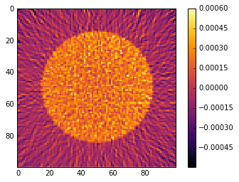
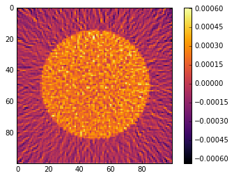
Take a look at the two noisy reconstructions.
plt.imshow(recA[0], cmap='inferno', interpolation="none")
plt.colorbar()
plt.savefig('UnitCircle_noise0.png', dpi=600,
        orientation='landscape', papertype=None, format=None,
        transparent=True, bbox_inches='tight', pad_inches=0.0,
        frameon=False)
plt.show()
plt.imshow(recB[0], cmap='inferno', interpolation="none")
plt.colorbar()
plt.show()
Calculate MTF
This metric is meaningful without noise. You can separate the MTF into
multiple directions or average them all together using the Ntheta
argument.
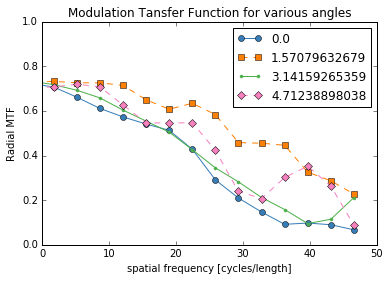
mtf_freq, mtf_value, labels = compute_mtf(p, recA[0], Ntheta=4)
The MTF is really a symmetric function around zero frequency, so usually people just show the positive portion. Sometimes, there is a peak at the higher spatial frequencies instead of the MTF approaching zero. This is probably because of aliasing noise content with frequencies higher than the Nyquist frequency.
plot_mtf(mtf_freq, mtf_value, labels)
plt.gca().set_xlim([0,50]) # hide negative portion of MTF
plt.show()
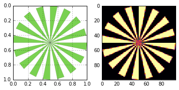
You can also use a Siemens Star to calculate the MTF using a fitted sinusoidal method instead of the slanted edges that the above method uses.
s = SiemensStar(n_sectors=32, center=Point([0.5, 0.5]), radius=0.5)
d = sidebyside(s, 100)
plt.show()
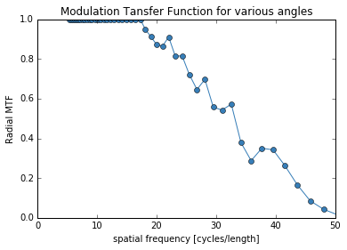
Here we are using the discreet verison of the phantom (without noise), so we are only limited by the resolution of the image.
mtf_freq, mtf_value = compute_mtf_siemens(s, d)
plot_mtf(mtf_freq, mtf_value, labels=None)
plt.gca().set_xlim([0,50]) # hide portion of MTF beyond Nyquist frequency
plt.show()
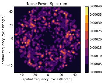
Calculate NPS
You can also calculate the radial or 2D frequency plot of the NPS.
X, Y, NPS = compute_nps(p, recA[0], plot_type='frequency',B=recB[0])
plot_nps(X, Y, NPS)
plt.show()
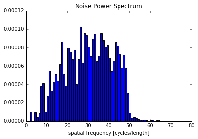
bins, counts = compute_nps(p, recA[0], plot_type='histogram',B=recB[0])
plt.figure()
plt.bar(bins, counts)
plt.xlabel('spatial frequency [cycles/length]')
plt.title('Noise Power Spectrum')
plt.show()
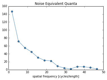
Calculate NEQ
freq, NEQ = compute_neq(p, recA[0], recB[0])
plt.figure()
plt.plot(freq.flatten(), NEQ.flatten())
plt.xlabel('spatial frequency [cycles/length]')
plt.title('Noise Equivalent Quanta')
plt.show()